Foundations of simple linear regression and getting started with Google Colab

Isai Guizar

Disclaimer:

This document is intended for educational purposes only. It does not constitute business advice.

This note reviews the foundations of econometric analysis through a simple financial application. Using Python in Google Colab, we will retrieve market data directly from Yahoo Finance, transform prices into returns, and estimate a simple Capital Asset Pricing Model (CAPM) regression. The exercise revisits the interpretation of coefficients, goodness of fit, hypothesis tests, and confidence intervals while introducing the reproducible computational workflow that will be used throughout the course.

1 Intro

Before studying models designed specifically for data ordered over time, it is useful to revisit the basic language of econometrics. In this session, we will estimate a simple linear regression using firm-level data and use the results to review four central ideas:

what estimated coefficients represent;
what the coefficient of determination, \(R^2\), measures—and what it does not measure;
how to formulate and interpret a hypothesis test;
how to construct and interpret a confidence interval.

At the same time, we will learn how to use Google Colab to write text, run Python code, examine results, and share a reproducible notebook.

Question

How sensitive is a stock’s return to movements in the overall market?

1.1 Types of data sets

The econometric methods we can use depend on the structure of the data.

Data structure	What we observe	Financial example
Cross section	Many units during the same period	ROE across different firms in 2025
Time series	One or more variables over time	Daily returns on Apple and the market
Panel data	The same units over time	Annual returns for several firms over ten years

In this session, data on each observation corresponds to a trading day. The data therefore form a time series. We will use familiar OLS tools to review econometric interpretation, but we will not assume that chronological order is irrelevant. Later in the course, we will examine temporal dependence, changing volatility, stationarity, and other features that require methods designed specifically for time-series data.

Important

A regression can be estimated with different data structures, but its assumptions and the appropriate method of inference depend on how the observations were generated. The use of inappropriate methods may lead to misleading results

1.2 Getting started with Google Colab

Google Colab allows you to run Python in a web browser without installing it on your computer.

Go to https://colab.research.google.com/.
Select New notebook.
Rename it Session_01.ipynb.
Identify the two types of cells:
- Text, for explanations, headings, and equations.
- Code, for Python instructions.
Run a cell by clicking the play button or pressing Shift + Enter.

Try this first instruction:

print("My first Time Series notebook")

My first Time Series notebook

Colab temporarily assigns a remote computer to the notebook. Variables and installed packages remain available during the session, but they may disappear when the runtime restarts. A reproducible notebook should therefore include all installation, import, data-retrieval, and transformation instructions from the beginning.

Two common mistakes

Running cells out of order may produce inconsistent results.
If the runtime restarts, select Runtime > Run all to rebuild the analysis.

2 Application: market risk and stock returns

We will estimate the market sensitivity of Apple Inc. using:

Yahoo Finance ticker	Role in the analysis	Variable
`AAPL`	Asset of interest	Apple return
`SPY`	Broad U.S. equity-market proxy, tracks the performance of the S&P 500	Market return
`^IRX`	13-week U.S. Treasury bill yield proxy	Risk-free rate

The stock and dates can be changed later without replacing the data source or rewriting the analysis.

Proxy variables

We use the SPY and ^IRX as practical proxies for the return on the complete market portfolio and a risk-free asset, so the estimated model we will develop is an empirical approximation to the theoretical CAPM.

2.1 Data

2.1.1 Prepare the environment

We now import the tools we need for this application

import numpy as np
import pandas as pd
import matplotlib.pyplot as plt
import seaborn as sns
import yfinance as yf
import statsmodels.formula.api as smf
from scipy import stats

sns.set_theme(style="whitegrid")
pd.set_option("display.float_format", lambda x: f"{x:,.4f}")

2.1.2 Retrieve the data

stock_ticker = "AAPL"
market_ticker = "SPY"
risk_free_ticker = "^IRX"

start_date = "2021-01-01"
end_date = "2026-01-01"

tickers = [stock_ticker, market_ticker, risk_free_ticker]

raw_data = yf.download(tickers, start=start_date, end=end_date, auto_adjust=True, progress=False, group_by="column"
)

raw_data.head()

Price	Close			High			Low			Open			Volume
Ticker	AAPL	SPY	^IRX	AAPL	SPY	^IRX	AAPL	SPY	^IRX	AAPL	SPY	^IRX	AAPL	SPY	^IRX
Date
2021-01-04	125.7409	342.4369	0.0680	129.8218	348.6210	0.0730	123.1660	338.7506	0.0680	129.7343	348.4910	0.0680	143301900	110210800	0
2021-01-05	127.2955	344.7954	0.0780	128.0048	345.8818	0.0800	124.7886	341.7498	0.0780	125.2356	341.7962	0.0780	97664900	66426200	0
2021-01-06	123.0105	346.8568	0.0780	127.3343	350.0417	0.0780	122.7967	342.7433	0.0780	124.0988	343.2912	0.0780	155088000	107997700	0
2021-01-07	127.2080	352.0102	0.0800	127.8979	352.7530	0.0830	124.2348	349.0482	0.0780	124.7206	349.2246	0.0780	109578200	68766800	0
2021-01-08	128.3060	354.0158	0.0800	128.8696	354.2294	0.0800	126.5376	350.1531	0.0800	128.6752	353.3937	0.0800	105158200	71677200	0

Yahoo Finance returns a two-level column index when several tickers are requested. We proceed to select the adjusted closing series and give them meaningful names.

prices = raw_data["Close"][[stock_ticker, market_ticker, risk_free_ticker]].copy()
prices.columns = ["stock_price", "market_price", "annual_rf_percent"]

prices.info()
prices.head()

<class 'pandas.core.frame.DataFrame'>
DatetimeIndex: 1255 entries, 2021-01-04 to 2025-12-31
Data columns (total 3 columns):
 #   Column             Non-Null Count  Dtype  
---  ------             --------------  -----  
 0   stock_price        1255 non-null   float64
 1   market_price       1255 non-null   float64
 2   annual_rf_percent  1255 non-null   float64
dtypes: float64(3)
memory usage: 39.2 KB

	stock_price	market_price	annual_rf_percent
Date
2021-01-04	125.7409	342.4369	0.0680
2021-01-05	127.2955	344.7954	0.0780
2021-01-06	123.0105	346.8568	0.0780
2021-01-07	127.2080	352.0102	0.0800
2021-01-08	128.3060	354.0158	0.0800

2.1.3 Inspect the price series

fig, axes = plt.subplots(3, 1, figsize=(7, 7), sharex=True)

prices["stock_price"].plot(ax=axes[0], color="steelblue")
axes[0].set(title=f"{stock_ticker} Adjusted Price", ylabel="USD")

prices["market_price"].plot(ax=axes[1], color="lightseagreen")
axes[1].set(title=f"{market_ticker} Adjusted Price", ylabel="USD")

prices["annual_rf_percent"].plot(ax=axes[2], color="tomato")
axes[2].set(title=f"{risk_free_ticker} Annualized Yield", ylabel="Percent", xlabel="Date")

plt.tight_layout()
plt.show()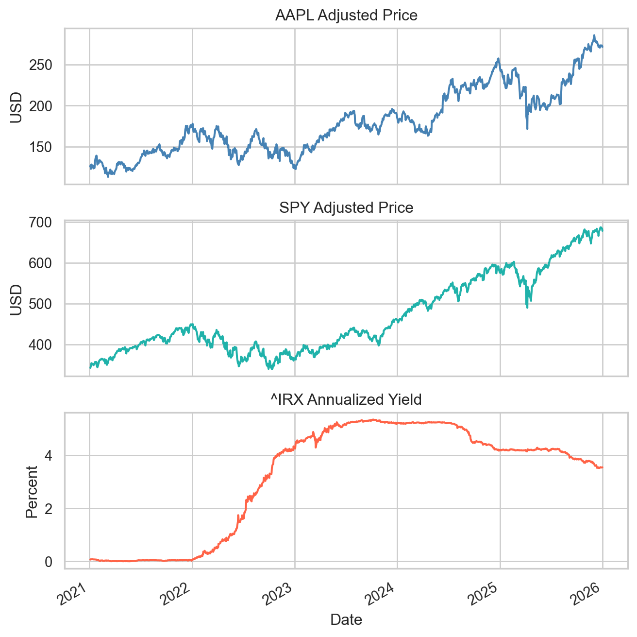

2.1.4 Estimate the returns

data = prices.copy()

data["stock_return"] = np.log(data["stock_price"]).diff() * 100
data["market_return"] = np.log(data["market_price"]).diff() * 100

The ^IRX series is an annualized yield expressed in percent. We approximate its daily effective return by:

\[ R_{f,t}^{daily} =100\left[\left(1+\frac{y_t}{100}\right)^{1/252}-1\right], \]

where 252 is the conventional approximate number of trading days in a year. The result is also measured in daily percentage points.

data["rf_return"] = 100 * (
    (1 + data["annual_rf_percent"] / 100)**(1 / 252) - 1
)

The CAPM regression can be expresses as:

\[ R_{i,t}-R_{f,t} =\alpha_i+\beta_i(R_{m,t}-R_{f,t})+u_t. \]

it uses excess returns, not raw returns:

data["stock_excess"] = data["stock_return"] - data["rf_return"]
data["market_excess"] = data["market_return"] - data["rf_return"]

capm_data = data[[
    "stock_return", "market_return", "rf_return",
    "stock_excess", "market_excess"
]].dropna()

print(f"First observation: {capm_data.index.min().date()}")
print(f"Last observation:  {capm_data.index.max().date()}")
print(f"Trading days:      {len(capm_data):,}")
capm_data.head()

First observation: 2021-01-05
Last observation:  2025-12-31
Trading days:      1,254

	stock_return	market_return	rf_return	stock_excess	market_excess
Date
2021-01-05	1.2288	0.6864	0.0003	1.2285	0.6861
2021-01-06	-3.4241	0.5961	0.0003	-3.4244	0.5958
2021-01-07	3.3554	1.4748	0.0003	3.3551	1.4745
2021-01-08	0.8594	0.5681	0.0003	0.8591	0.5678
2021-01-11	-2.3523	-0.6764	0.0003	-2.3527	-0.6767

2.1.5 Descriptive statistics

capm_data.describe().T

	count	mean	std	min	25%	50%	75%	max
stock_return	1,254.0000	0.0613	1.7490	-9.7013	-0.7965	0.1095	0.9795	14.2617
market_return	1,254.0000	0.0545	1.0762	-6.0326	-0.4531	0.0746	0.6286	9.9863
rf_return	1,254.0000	0.0125	0.0080	0.0000	0.0021	0.0163	0.0196	0.0207
stock_excess	1,254.0000	0.0489	1.7489	-9.7176	-0.8046	0.0968	0.9727	14.2453
market_excess	1,254.0000	0.0420	1.0760	-6.0488	-0.4640	0.0588	0.6138	9.9699

Remember that all returns are measured in daily percentage points. A value of 1.25 means 1.25%, not 125%.

2.1.6 Visualize returns over time

fig, axes = plt.subplots(2, 1, figsize=(7, 7), sharex=True)

capm_data["stock_return"].plot(ax=axes[0], color="steelblue", linewidth=0.8)
axes[0].axhline(0, color="black", linewidth=0.8)
axes[0].set(title=f"Daily {stock_ticker} Returns", ylabel="Percent")

capm_data["market_return"].plot(ax=axes[1], color="lightseagreen", linewidth=0.8)
axes[1].axhline(0, color="black", linewidth=0.8)
axes[1].set(title=f"Daily {market_ticker} Returns", ylabel="Percent", xlabel="Date")

plt.tight_layout()
plt.show()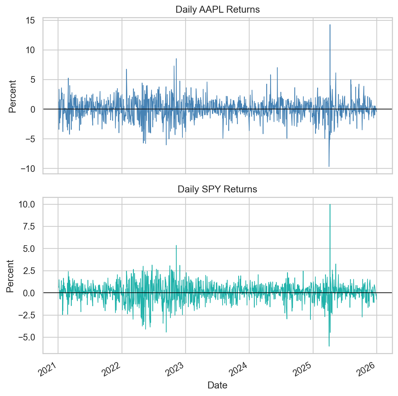

2.2 The CAPM regression

The theoretical CAPM states that expected excess returns satisfy

\[ E(R_i)-R_f=\beta_i[E(R_m)-R_f]. \]

A common empirical time-series specification is

\[ R_{i,t}-R_{f,t} =\alpha_i+\beta_i(R_{m,t}-R_{f,t})+u_t. \]

In this application:

\(R_{i,t}-R_{f,t}\) is Apple’s daily excess return;
\(R_{m,t}-R_{f,t}\) is the daily excess return on SPY;
\(\alpha_i\) measures average abnormal excess return not explained by the market;
\(\beta_i\) measures the stock’s sensitivity to market movements;
\(u_t\) contains firm-specific news and other influences not captured by the market.

CAPM regression versus market model

The market model regresses the stock’s raw return on the market’s raw return. The empirical CAPM instead uses excess returns on both sides. When the daily risk-free return is small, the numerical estimates may be similar, but the models are conceptually different.

fig, ax = plt.subplots(figsize=(7, 7))

sns.regplot(
    data=capm_data,
    x="market_excess",
    y="stock_excess",
    ci=None,
    scatter_kws={"alpha": 0.75, "s": 30},
    line_kws={"color": "#c43d3d", "linewidth": 0.5},
    ax=ax
)

ax.set(
    title=f"{stock_ticker} and Market Excess Returns",
    xlabel="Market Excess Return (%)",
    ylabel=f"{stock_ticker} Excess Return (%)"
)
plt.show()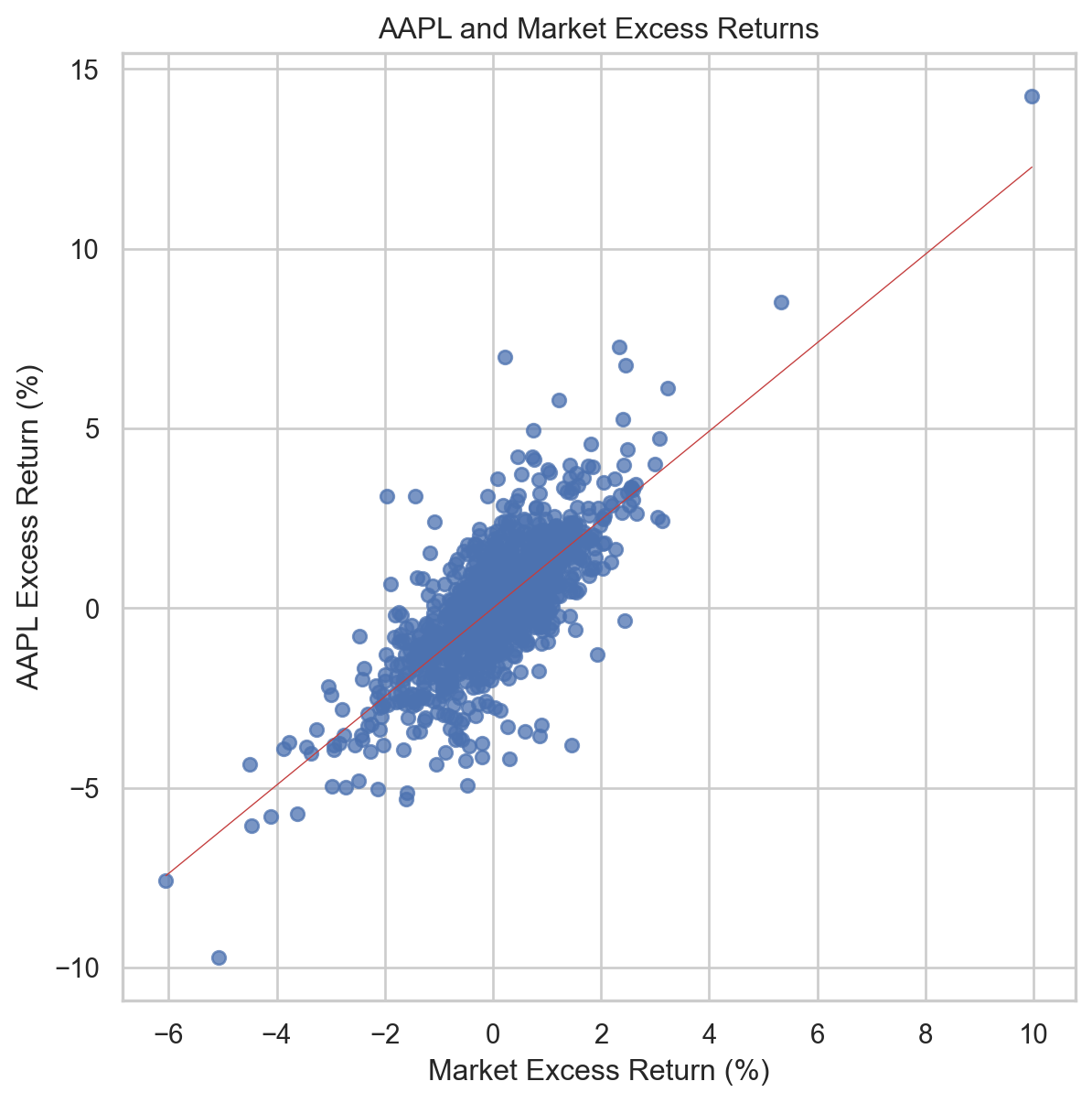

Observe:

Does the plot suggest a positive or negative relationship?
Does the fitted line appear steep or flat?
Are there observations that could substantially influence the fitted line?
Is the graph alone sufficient to establish that market movements cause every change in the stock?

2.3 Estimation by ordinary least squares (OLS)

OLS chooses \(\widehat{\alpha}\) and \(\widehat{\beta}\) to minimize

\[ \sum_{t=1}^{T} \left[(R_{i,t}-R_{f,t}) -\widehat{\alpha} -\widehat{\beta}(R_{m,t}-R_{f,t})\right]^2. \]

capm = smf.ols("stock_excess ~ market_excess", data=capm_data).fit()
print(capm.summary())

                            OLS Regression Results                            
==============================================================================
Dep. Variable:           stock_excess   R-squared:                       0.574
Model:                            OLS   Adj. R-squared:                  0.573
Method:                 Least Squares   F-statistic:                     1684.
Date:                Wed, 05 Aug 2026   Prob (F-statistic):          5.67e-234
Time:                        13:10:08   Log-Likelihood:                -1945.4
No. Observations:                1254   AIC:                             3895.
Df Residuals:                    1252   BIC:                             3905.
Df Model:                           1                                         
Covariance Type:            nonrobust                                         
=================================================================================
                    coef    std err          t      P>|t|      [0.025      0.975]
---------------------------------------------------------------------------------
Intercept        -0.0029      0.032     -0.089      0.929      -0.066       0.060
market_excess     1.2310      0.030     41.037      0.000       1.172       1.290
==============================================================================
Omnibus:                      107.415   Durbin-Watson:                   1.816
Prob(Omnibus):                  0.000   Jarque-Bera (JB):              620.715
Skew:                           0.073   Prob(JB):                    1.63e-135
Kurtosis:                       6.444   Cond. No.                         1.09
==============================================================================

Notes:
[1] Standard Errors assume that the covariance matrix of the errors is correctly specified.

We can extract the results that we will use most often.

results = pd.DataFrame({
    "coefficient": capm.params,
    "standard_error": capm.bse,
    "t_statistic": capm.tvalues,
    "p_value": capm.pvalues
})

results

	coefficient	standard_error	t_statistic	p_value
Intercept	-0.0029	0.0323	-0.0890	0.9291
market_excess	1.2310	0.0300	41.0372	0.0000

The estimated equation is

\[ \widehat{R_{i,t}-R_{f,t}} =\widehat{\alpha} +\widehat{\beta}(R_{m,t}-R_{f,t}). \]

alpha_hat = capm.params["Intercept"]
beta_hat = capm.params["market_excess"]

print(
    f"Predicted stock excess return = {alpha_hat:.4f} "
    f"+ {beta_hat:.4f} × market excess return"
)

Predicted stock excess return = -0.0029 + 1.2310 × market excess return

2.3.1 Interpret the coefficients

The slope (beta)

\(\widehat{\beta}\) is the estimated change in the stock’s daily excess return associated with a one-percentage-point increase in the market’s daily excess return.

If the market excess return increases by one percentage point, the stock’s excess return is predicted to change by \(\widehat{\beta}\) percentage points, on average.

A conventional interpretation is:

\(\beta>1\): the stock tends to move more than the market;
\(0<\beta<1\): the stock tends to move in the same direction, but less than the market;
\(\beta<0\): the stock tends to move in the opposite direction.

These are sensitivity interpretations, not guarantees about the return on any individual day.

The constant (alpha)

\(\widehat{\alpha}\) is the predicted daily stock excess return when the market excess return equals zero. Under the CAPM, the population alpha should equal zero:

\[ H_0:\alpha=0. \]

A statistically nonzero alpha may reflect abnormal performance, but it may also result from sampling variation, an inadequate market proxy, changing beta, omitted risk factors, or model misspecification.

2.3.2 Fitted values and residuals

For each trading day:

\[ \widehat{u}_t =(R_{i,t}-R_{f,t}) -\widehat{(R_{i,t}-R_{f,t})}. \]

capm_results = capm_data.copy()
capm_results["fitted_excess_return"] = capm.fittedvalues
capm_results["residual"] = capm.resid

capm_results.head()

	stock_return	market_return	rf_return	stock_excess	market_excess	fitted_excess_return	residual
Date
2021-01-05	1.2288	0.6864	0.0003	1.2285	0.6861	0.8416	0.3868
2021-01-06	-3.4241	0.5961	0.0003	-3.4244	0.5958	0.7305	-4.1549
2021-01-07	3.3554	1.4748	0.0003	3.3551	1.4745	1.8122	1.5429
2021-01-08	0.8594	0.5681	0.0003	0.8591	0.5678	0.6961	0.1630
2021-01-11	-2.3523	-0.6764	0.0003	-2.3527	-0.6767	-0.8358	-1.5168

A positive residual means the stock outperformed the model’s prediction that day.
A negative residual means the stock underperformed the prediction.
With an intercept, OLS residuals sum to approximately zero.

capm_results["residual"].sum()

-8.526512829121202e-14

2.4 Goodness of fit: \(R^2\)

The \(R^2\) is the proportion of the sample variation in the dependent variable (stock’s excess returns) explained by the model – their linear relationship with market excess returns:

\[ R^2=1-\frac{\sum_t \widehat{u}_t^2} {\sum_t[(R_{i,t}-R_{f,t})-\overline{(R_i-R_f)}]^2}. \]

y = capm_data["stock_excess"]
y_hat = capm.fittedvalues
residuals = capm.resid

TSS = ((y - y.mean())**2).sum()
ESS = ((y_hat - y.mean())**2).sum()
RSS = (residuals**2).sum()
R2_manual = 1 - RSS / TSS

print(f"TSS: {TSS:,.4f}")
print(f"ESS: {ESS:,.4f}")
print(f"RSS: {RSS:,.4f}")
print(f"R²:  {R2_manual:.4f}")

TSS: 3,832.6950
ESS: 2,198.3458
RSS: 1,634.3492
R²:  0.5736

What R² does not establish

A high \(R^2\) does not establish that the CAPM is the correct asset-pricing model, and it does not imply that the market explains every daily movement. A low \(R^2\) does not imply that beta is irrelevant: firm-specific news can generate substantial residual variation.

2.5 Hypothesis tests

2.5.1 Is beta statistically different from zero?

\[ H_0:\beta=0 \qquad \text{versus} \qquad H_1:\beta\neq0. \]

The statistic is

\[ t=\frac{\widehat{\beta}-0}{se(\widehat{\beta})}. \]

se_beta = capm.bse["market_excess"]
t_beta = capm.tvalues["market_excess"]
p_beta = capm.pvalues["market_excess"]

print(f"Beta:           {beta_hat:.4f}")
print(f"Standard error: {se_beta:.4f}")
print(f"t statistic:    {t_beta:.4f}")
print(f"p-value:        {p_beta:.4g}")

Beta:           1.2310
Standard error: 0.0300
t statistic:    41.0372
p-value:        5.672e-234

The \(p\)-value is the probability, assuming the null hypothesis and the model’s assumptions are true, of obtaining a test statistic at least as extreme as the one observed.

2.5.2 Does the stock have the same market sensitivity as the market?

This is the test

\[ H_0:\beta=1 \qquad \text{versus} \qquad H_1:\beta\neq1. \]

test_beta_one = capm.t_test("market_excess = 1")
print(test_beta_one)

                             Test for Constraints                             
==============================================================================
                 coef    std err          t      P>|t|      [0.025      0.975]
------------------------------------------------------------------------------
c0             1.2310      0.030      7.700      0.000       1.172       1.290
==============================================================================

2.5.3 Is alpha different from zero?

p_alpha = capm.pvalues["Intercept"]

print(f"Alpha:   {alpha_hat:.4f}% per trading day")
print(f"p-value: {p_alpha:.4f}")

Alpha:   -0.0029% per trading day
p-value: 0.9291

Decision rule for a significance level \(\alpha_s\):

if the \(p\)-value is less than \(\alpha_s\), reject \(H_0\);
otherwise, do not reject \(H_0\).

Use precise language

Failing to reject \(H_0\) does not prove that the parameter equals the null value. It means that the sample does not provide sufficient evidence to reject that value at the selected significance level.

2.6 Confidence intervals

A 95% confidence interval for beta is

\[ \widehat{\beta} \pm t_{0.025,\,T-2}\,se(\widehat{\beta}). \]

ci_95 = capm.conf_int(alpha=0.05)
ci_95.columns = ["lower_bound", "upper_bound"]
ci_95

	lower_bound	upper_bound
Intercept	-0.0662	0.0605
market_excess	1.1721	1.2898

We can verify the interval for beta manually.

degrees_freedom = int(capm.df_resid)
critical_t = stats.t.ppf(0.975, df=degrees_freedom)

lower_beta = beta_hat - critical_t * se_beta
upper_beta = beta_hat + critical_t * se_beta

print(f"Critical value: {critical_t:.4f}")
print(f"95% CI for beta: [{lower_beta:.4f}, {upper_beta:.4f}]")

Critical value: 1.9619
95% CI for beta: [1.1721, 1.2898]

A careful frequentist interpretation is:

If we repeatedly obtained samples and constructed an interval using this procedure, approximately 95% of those intervals would contain the true parameter.

For the sample at hand, the interval reports the values of beta that are reasonably compatible with the data and model at the 5% significance level.

2.7 Assumptions and time-series limitations

The familiar simple-regression assumptions still matter, but their interpretation changes when observations are ordered over time:

Linearity in parameters: the model is linear in alpha and beta.
Random Sampling: the data is a random sample drawn from the population
No perfect collinearity: market excess returns vary in the sample.
Zero conditional mean: \(E(u_t\mid R_{m,t}-R_{f,t})=0\).
Constant variance: conventional standard errors assume homoskedastic errors.
No serial correlation: conventional time-series inference assumes residuals are not correlated across dates.

Daily financial returns commonly exhibit volatility clustering, so constant conditional variance may be unrealistic. Residual dependence or changing beta can also affect conventional inference. These are not side issues: they motivate later topics in the course.

3 Practice

Choose one publicly traded company other than Apple and replace AAPL with its Yahoo Finance ticker. Keep SPY and ^IRX as the market and risk-free proxies.

Submit a Google Colab link containing:

a brief cover section with the team members’ names and selected company;
all cells executed in order;
a price graph and a return graph;
the scatterplot with the fitted regression line;
the OLS results and the 95% confidence intervals;
a conclusion of no more than 150 words distinguishing market sensitivity, explanatory power, statistical significance, and model limitations.

3.1 what changes with time-series data?

The mechanics of simple OLS remain familiar, but today’s observations were trading days rather than independent firms. Their ordering matters because:

returns may depend on past information;
volatility can cluster over time;
parameters such as beta may change;
residuals may be serially correlated;
prices and other persistent variables can produce spurious regressions when used in levels.

The transformation from prices to returns was therefore not merely a coding step. It was our first econometric decision based on the time-series structure of the data.

4 References

Guizar, I. (2026). Introductory Econometrics in Python. Chapters 1 and 2. https://i-guizar.quarto.pub/introductory-econometrics-in-python/
Sharpe, W. F. (1964). Capital asset prices: A theory of market equilibrium under conditions of risk. The Journal of Finance, 19(3), 425–442.
Wooldridge, J. M. (2020). Introductory Econometrics: A Modern Approach (7th ed.). Cengage Learning, Chapters 2 and 10.
Yahoo Finance historical market data, retrieved programmatically with the yfinance Python package.